Consider an import service that validates uploaded records, transforms them, and streams results back to callers. We instrument the service with OpenTelemetry to capture traces, metrics, and logs.
Traces capture the execution flow and relationships between operations. Metrics track request counts and processing durations, while logs record individual events and diagnostic details. Each signal provides a different view of the same application.
To control telemetry volume, developers sample traces, configure metric aggregation, filter logs, and batch exports. These mechanisms reduce the amount of data recorded, retained, or transmitted at different stages. But they do not necessarily eliminate the work that happens before those stages.
A dropped span may still require the application to construct attributes. A metric may produce only a few exported data points while its aggregation state occupies memory. A batched log may still require formatting and processing on the application thread before reaching a queue.
Some of these costs consume CPU during application execution. Others persist as memory allocations, queued work, or background processing. They are not always visible in the telemetry that eventually reaches a backend.
Less telemetry leaving a process does not necessarily mean less instrumentation work.
This raises the question explored throughout the article: What work and state remain inside an instrumented application, and where do the other costs move?
OpenTelemetry defines common APIs and behavioral contracts across languages, but SDK implementations differ. We will use the specification to explain shared behavior and examine implementation details where they matter. Most implementation examples use OpenTelemetry Python SDK 1.45.1, with selected examples from Go and Node.js. Findings from one implementation should not be treated as universal SDK guarantees.
Here is the distinction to keep in mind as we follow the pipeline:
| Mechanism | What it can reduce | What can remain |
|---|---|---|
| Head sampling | Recording and export of dropped spans | Caller inputs, identity and sampler work |
| Tail sampling | Downstream trace volume | Upstream recording/export, trace buffers |
| Metric aggregation | Per-measurement export volume | Recording-time updates, aggregation state |
| Bound instruments, where supported | Repeated attribute processing and lookup | Aggregation updates, bound-handle state |
| Batch export | Caller waiting for export | Queue admission, buffering, worker work |
Reducing telemetry volume, reducing application overhead and reducing total system cost are three different optimization goals.
1. What happens when you create a span?
The import handler wants a job span with a cheap job.kind attribute and
detailed diagnostics about the submitted records. Sampling seems like the
obvious way to control the expense. To understand what it can save, follow
the call from the application into the SDK.
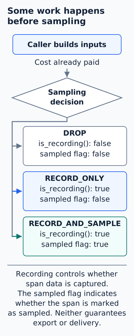
Inputs come before the sampling decision
The application first prepares the arguments it will pass to the tracing API. If those arguments require walking a collection, converting values, or building a diagnostic string, that work belongs to the caller. The sampler has not been consulted yet.
In tracer.start_span("job", attributes=build_all_attributes()), Python runs
build_all_attributes() before calling start_span. By the time the SDK
receives the attributes, their construction cost has already been paid.
Sampling cannot undo that work.
The SDK determines the span's parent and trace identity. The sampler then uses the available parent context, span name, initial attributes, and links to decide whether the span should be recorded and marked as sampled.
The trace SDK specification requires SDKs to behave as if they establish the trace ID, consult the sampler, then generate a span ID independently of the decision. SDKs need not perform identical instructions or allocations to satisfy that contract.
Even a dropped span can retain valid trace and span identifiers for context propagation. Dropping its recording does not eliminate the earlier work of resolving parent context, establishing identity, or making the sampling decision.
The result is either a recording span, which accepts span data for processing, or a non-recording span, which ignores recording operations. Recording spans may invoke processors at creation and ending, depending on the processor contract.
Choosing not to record avoids subsequent recording work. It cannot undo the work the application already performed to create the span.
Why record a span that is not sampled?
Exporting a trace is not the only use of span data. A processor may need information about operations to derive local metrics without sending every span onward as trace data. The specification describes span-to-metrics processing as a use for recording spans that would otherwise be dropped. That processing still costs CPU and needs recording state; it must also be configured rather than assumed to happen automatically.
Recording and sampling are separate properties. Recording determines whether
the span accepts data for processing, while the sampled flag indicates its
sampling status. RECORD_ONLY records span data without marking the span as
sampled. Unlike DROP, it still incurs recording costs.
The three sampler outcomes express that distinction. DROP produces a non-recording span with the sampled flag unset. RECORD_ONLY produces a recording span with the flag unset. RECORD_AND_SAMPLE records and sets the flag. Standard export processing uses that flag: the trace specification says unsampled spans SHOULD NOT be exported, not that every custom processor is forbidden from using their data.
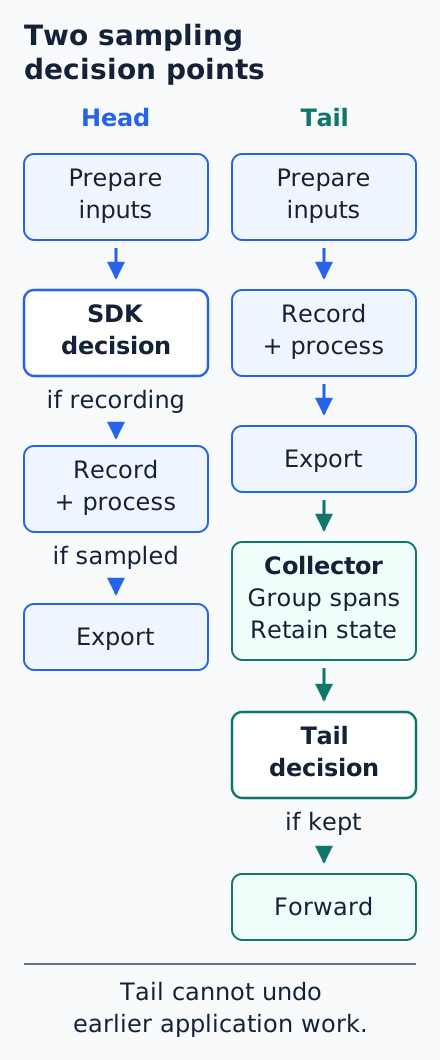
Head sampling and tail sampling: when the decision happens matters
Suppose the import service processes 10,000 requests, but only a few fail. Head sampling can reduce recording cost, but may discard a request before knowing it will fail. Tail sampling can select traces using their eventual outcome, provided candidate spans were recorded and delivered to the sampling component.
Head sampling decides when a span starts, using information such as the parent context, span name and initial attributes. DROP can avoid subsequent recording and processor work. It cannot undo caller-side input construction or consider an operation's eventual failure or latency before those events have occurred.
Tail sampling postpones selection until trace data has been observed. It can use errors, durations and attributes recorded during execution rather than relying only on information available at the start. The additional information can make selection better informed, but is not free.
In a common SDK-to-Collector deployment, the application pays to record, process and export candidate spans; the Collector pays to group, buffer and evaluate traces. Discarding spans before backend ingestion cannot recover that earlier application work. Tail sampling also cannot recover spans that an upstream head sampler never recorded or sent.
The Collector's tail-sampling processor groups spans by trace ID and retains state while making decisions. When this processor runs across multiple Collector instances, spans from the same trace need to reach the same instance so the decision can consider them together. That routing requirement belongs to this stateful implementation, not every possible sampling architecture.
A tail decision need not wait for every span. The sampling component needs policies for incomplete traces, late arrivals, decision timeouts and memory limits. A waiting period expiring does not prove a trace is complete.
The trade-off is therefore not just the fraction retained. Head sampling can avoid recording early; tail sampling can reduce backend volume, but cannot undo work already paid for by the application or Collector.
Sources: Specification 1.62.0 span creation; Collector Contrib 0.164.1 decision policies.
Put the guard before optional enrichment
Back at the SDK's span-creation boundary, the application can ask whether the span is recording. This reflects the local decision, not a future tail-sampling outcome. It is the useful gate for expensive optional detail: can this span use the value, not will a backend eventually receive it? Checking only the sampled flag would also skip work for RECORD_ONLY spans.
OpenTelemetry also defines an Enabled API for
tracers,
synchronous metric instruments,
and loggers.
Where supported, it lets instrumentation check whether telemetry is enabled
before constructing expensive inputs. Unlike span.is_recording(), which
checks an existing span, Tracer.Enabled can avoid unnecessary work before
span creation. It does not predict the sampling decision for an individual
span. Availability depends on the language implementation.
There is still an eager-evaluation boundary at each later method call.
This Python excerpt assumes an already-created span and an application
build_diagnostics():
span.set_attribute("diagnostics", build_diagnostics())The application evaluates build_diagnostics() before calling the setter.
A non-recording span can ignore the result, but it cannot prevent the
construction. Put the recording predicate around the
optional work instead. This excerpt assumes a configured tracer, plus
build_diagnostics() and do_work():
span = tracer.start_span("job", attributes={"job.kind": "import"})
try:
    if span.is_recording():
        span.set_attribute("diagnostics", build_diagnostics())
    do_work()
finally:
    span.end()
The guard avoids optional work after creation. It cannot avoid constructing
attributes already passed into start_span. Keep necessary head-sampler
inputs, such as job.kind, cheap and available at creation: enrichment added
later cannot influence a decision already made.
Creating a span does not automatically make it current. To let subsequent
instrumentation discover it as the parent, activate it around the relevant
work. Ending the span closes its recording lifecycle and can invoke processors.
A simple processor may export inline, while a batch processor can queue the
span for later export. Some work therefore happens during end(), while
other work may continue afterward.
A span's duration is not a measure of its instrumentation overhead. In Python SDK 1.45.1, some recording state is created before the default start timestamp, while end processors run after the end timestamp is set. The span's duration therefore excludes some work involved in creating and ending it. Measuring instrumentation overhead requires observing that work separately.
An attribute limit is not a limit on attribute work
Suppose a span has a limit of ten attributes, and one contains a list of 1,000 identifiers. It counts as one key, but the SDK may need to validate and copy the whole list. Replace that attribute as the import progresses, and the work can repeat without increasing the number of retained keys.
An attribute-count limit controls how many keys are retained, not how much work is required to process each value.
Copying is also an ownership decision. The import handler can continue modifying its list after assigning it to a span. If the SDK retained that mutable list directly, a later reader could see changes made after the assignment. Taking a snapshot separates the application's live data from the value the instrumentation intended to record.
Python SDK 1.45.1's attribute implementation, for example, walks a sequence and converts it to a tuple. With a positive key-count limit, that happens before insertion or replacement. Assigning an equivalent list again does not tell this path that validation and copying can be skipped.
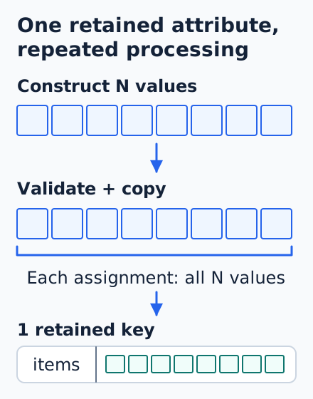
The stored tuple remains isolated from later changes to the caller's list.
Bound value sizes as well as key counts. Reusing an immutable input can avoid caller construction, but does not make the SDK skip validation or copying. Check the ownership contract before reusing mutable containers.
Sources: Python API/SDK 1.45.1 value cleaning and attribute insertion/replacement.
Instrument handles are not free to acquire
Before creating a span or recording a metric, instrumentation needs a handle. A helper that obtains a tracer, meter or counter on every request can put acquisition work back on the hot path, even when the provider caches handles. Returning an existing object is not the same as doing no work to find it.
For example, Python SDK 1.45.1 constructs instrumentation metadata and a scope object, then enters a locked registry lookup. The provider may return a cached tracer, but constructing lookup metadata and finding that tracer still require work.
Use stable instrumentation scope names and acquire handles at the application, library or component lifetime that owns them. A cached tracer lookup is a different operation from creating a span. Unique instrument names introduce a separate retained-state problem, which becomes clearer when we follow a metric into its aggregation storage.
2. Why fewer metrics don't always mean less memory
The import service records a completed request with a counter. It needs an outcome dimension, but someone also adds a request identifier to help with diagnosis.
For this counter, each distinct attribute combination can create a separate time series. Cardinality is the number of these series. A unique request ID can therefore produce one series per request, even when the counter name and outcome stay the same.
The complete identity also includes the resource being observed, the instrumentation scope and properties of the metric stream. A View configures that stream's attributes and aggregation; the metric data model describes the full identity rules.
Three counts matter: distinct attribute combinations arriving over time, aggregation entries retained by the SDK, and points in an export. They need not move together. To see why, separate what a collection represents from what the SDK must keep between collections.
Delta changes the interval represented
A reader collects metric data for consumption or export. Its temporality describes the time range represented by that data. Cumulative output represents accumulation from a start time; delta output represents changes over a collection interval.
Consider a counter receiving 1,000 new identities in each of three intervals, without revisiting the old identities. A cumulative stream that keeps those identities can report 1,000 points, then 2,000, then 3,000: the old identities still have accumulated values. Delta output can report just the 1,000 identities updated in each interval.
That is the output pattern in the Python SDK 1.45.1 counter example. It does not tell us whether the old identities were deleted from memory. "No new value to export" and "no object retained for this identity" are different states.
What an aggregation entry contains
A counter call is not necessarily a small message waiting to be exported. With SDK-side aggregation, it can update a summary already living inside the process. Rather than preserve every increment as a separate record, the SDK finds the state associated with that measurement's identity and updates it. Repeated measurements can then become a much smaller collection of points.
In the inspected Python SDK 1.45.1 storage, that lookup uses a dictionary.
Measurements with the same selected attributes update the same entry; a new
combination creates another. With id retained, changing it creates another
key even when both calls have ok=True.
The instrument, matching View and reader determine which storage receives the measurement. Attributes do not form one global dictionary shared by every metric in the process.
For a synchronous Counter, the entry holds the sum being accumulated, the attributes needed to identify the resulting point, and collection-related state such as timestamps. The sum update is protected by the aggregation's lock. A histogram has different state, including bucket counts; an aggregation entry is not a fixed-size, universal unit of memory.
Identifying and updating this state happens when the application records a measurement. Collection does not retroactively perform that work on a background thread.
Bound instruments: moving lookup work out of the recording path
Bound instruments are an emerging OpenTelemetry Metrics API feature. The Bind API is marked Development in specification 1.62.0 and is optional for synchronous instruments; availability depends on the SDK.
Aggregation combines measurements into shared state, but the recording path
must first find the state to update. Consider the import service counting
processed records with stable job.kind=import and outcome=success
attributes. Repeatedly supplying them may repeat attribute processing and
aggregation lookup even though every increment belongs to the same series.
A bound instrument associates an attribute set with a reusable recording handle. Instead of resolving that identity on every call, the application binds once and records through the handle.
Where implemented, the SDK contract requires attribute processing and cardinality evaluation at bind time. Subsequent recordings without extra attributes must bypass the per-recording aggregation-map lookup.
Binding moves work rather than eliminating aggregation. Each recording still updates aggregation state and may require synchronization. Recordings that supply additional attributes may still require attribute processing and lookup, reducing the benefit of binding for those calls.
Binding is most useful when many measurements share the same attributes. If every measurement uses a different request ID, repeatedly creating bound handles simply moves work from recording to binding and can introduce additional retained state.
Views and binding solve different problems: Views determine which attributes identify an aggregation; binding optimizes repeated recording against the resolved identity. Neither makes high cardinality free.
Bind support and handle-lifecycle behavior vary across SDKs. The Python SDK examples in this article do not demonstrate Bind.
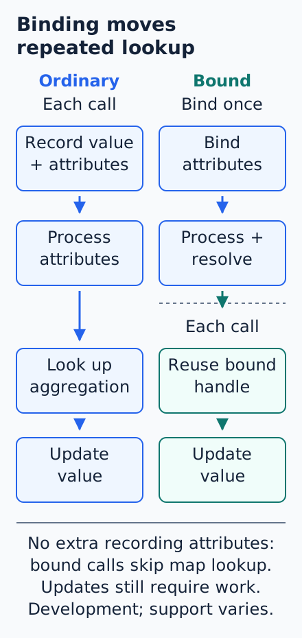
Sources: Specification 1.62.0 Bind API and SDK bind requirements. The SDK contract also requires bound recordings to remain candidates for exemplar sampling using each recording's context.
Bound instruments address the cost of repeatedly finding aggregation state. They do not determine how long that state remains in memory. That is a separate question, especially when attribute combinations change over time.
Collection is not the same as reclamation
In the Python SDK 1.45.1 storage path, collection walks the stored aggregation objects and asks each for a point. The synchronous sum's delta path takes the current interval's value and clears it to "no measurement." An entry with no new value can return no point. The surrounding dictionary, however, does not remove that entry.
The cumulative path carries a running total forward and can produce a point for an old identity even when no increment arrived in the current interval. Resetting a value or omitting it from an export does not release the aggregation entry. In the inspected Python SDK, the dictionary continues to retain that entry.
In the inspected Python SDK 1.45.1, the three-interval example retained 3,000 aggregation entries under both temporalities. Delta reduced the number of exported points, but did not remove the old entries. Even an idle collection still traversed the retained aggregation state without producing new delta points.
Garbage collection cannot reclaim entries that the SDK still owns through its map. Nor does discarding each exported snapshot release the separate aggregation objects that produced it. Reclaiming those objects requires an implementation policy, not just a choice of output temporality.
For a service with identity churn, today's small delta export can coexist with a larger working set inherited from earlier requests. Inspect the lifetime of the identity map, not just the point count at the exporter. The retained-map behavior belongs to this implementation; delta temporality does not require every SDK to keep old entries indefinitely.
Sources: Python SDK 1.45.1 collection over retained entries and sum reset versus cumulative accumulation.
Filtering changes the identity stored
The import service can address the cause earlier: change which attributes identify the aggregate. A View can retain the outcome dimension while discarding the per-request identifier before an aggregation entry is looked up or created. That changes the number of distinct entries the measurements can create, rather than merely changing which points appear at collection.
The inspected Python path filters attributes before computing the aggregation key. After the View removes the request ID, measurements with different IDs but the same outcome update one entry. The SDK still records every increment, but no longer creates a separate entry for every request.
When all measurements share ok=True after filtering, they update one
aggregation entry and produce one aggregated point. A service reporting
success and failure would retain separate outcome identities.
The trade-off is information, not just memory. After removing id, the
aggregate no longer provides a per-request-ID breakdown. If the operational
question is the request count by outcome, that loss of detail is intentional.
If individual request diagnosis is required, it needs a signal that retains
that detail rather than an unbounded identifier accidentally attached to
every metric measurement.
Filtering attributes and choosing the aggregation are separate View decisions. The filter determines which inputs share an identity; the aggregation determines what state summarizes them. Removing labels later in a Collector may reduce downstream series, but cannot undo the application's earlier dictionary insertions, sum updates or retained entries.
The View changes which measurements share an aggregate; it does not reduce how many measurement calls the application makes. Constructing and passing an attribute that the View will discard can still cost caller time. Keep that distinction when choosing between normalizing instrumentation inputs and filtering them inside the SDK.
Budget the state behind the stream
Cardinality limits are SDK-specific controls, not a universal memory budget. Where a limit is available, check what it bounds, how overflow is represented and which storage instances it applies to. For Python SDK 1.45.1, the inspected View and reader APIs do not expose a configurable metric-cardinality limit. The inspected insertion path does not apply an automatic 2,000-series cap. Bound attribute domains or filter them before aggregation rather than assuming another SDK's protection is present.
State also has owners beyond a single stream. A reader is not necessarily just another consumer looking at one shared snapshot. In the inspected implementation, synchronous measurements pass through each reader's storage, and each reader owns its aggregation entries. Adding a reader can therefore add state and update work, not just another destination for the same bytes.
Histogram bucket counts and additional instruments add other dimensions to the budget. Even where a series limit is available, a count of series cannot describe the byte size of every aggregation object, reader and export queue.
Instrument registries introduce another identity space. Moving a request ID from an attribute into a newly named counter does not remove the growth problem: the provider may retain a new instrument for every name. In the inspected Python implementation, creating counters with distinct names can grow the instrument registry even if those counters never record measurements. Registration state exists before aggregation sees its first measurement.
Use stable instrument and scope names, then budget the remaining attribute domains, aggregation detail and reader state. Exported series count describes the output; it is not a ceiling on everything the process retains.
Who executes an observable callback?
Suppose the import service wants to report how many jobs are currently waiting. It registers a callback that reads the current queue size when metrics are collected, rather than maintaining a second running total on every enqueue and dequeue.
An observable instrument asks that function for observations during collection. In the inspected Python path, the SDK invokes the callback and iterates its results wherever the reader schedules collection. The word asynchronous describes this instrument model, not a promise of a dedicated worker.
If obtaining the queue size requires a slow query or I/O, collection has to wait for that application work. Reading must also leave the observed state intact.
A callback that sums and clears a list illustrates the ownership problem: the first reader consumes state that the next reader also needs to observe. Collection order then changes the values. Reading a snapshot instead keeps collection as observation rather than consumption.
Different readers can collect separately, so a callback may run more than once for the same application state. The metric callback contract asks callbacks to be reentrant and not take an indefinite amount of time. These are callback responsibilities, not a universal interruption mechanism.
When obtaining a value requires I/O, give that I/O an independently owned task and transport deadline, then publish a bounded snapshot for collection. Decide how stale or unavailable values are represented. A collection deadline does not, by itself, cancel arbitrary application code or its transport.
3. The invisible cost of context propagation
A span can exist without being the current span. Creating a span establishes its identity and parent relationship, but it does not automatically make that span the parent of subsequent operations.
For subsequent instrumentation to discover a span as its parent automatically, that span must be made current in the execution context. Instrumentation can also supply an explicit parent context instead. How context travels across execution boundaries depends on the language and runtime.
Consider our import service. A producer transforms records and streams them to a consumer, which writes the response. We want the producer's transformation work to appear under a producer span, while the consumer's response-writing work remains under the outer request span.
This requires careful control over when the producer span becomes current and when the previous context is restored. Creating, activating, and ending a span are separate operations. Ending a span stops recording, but does not automatically restore the previous context or release references held elsewhere.
A scope can survive suspension
A producer activates its span, processes an item and yields a result from inside the activation's scope. Execution has left the producer, but the scope has not exited. If the consumer resumes with that same current context, its next span can inherit the producer rather than the outer request.
The surprise is the difference between suspension and scope exit. A block that looks local in one function can remain active while another function runs. Whether that context crosses the handoff depends on the runtime and how the work is scheduled; this is not a rule about every asynchronous call.
The Python SDK 1.45.1 example makes the boundary concrete. The consumer calls
await anext(generator) with the outer request current. The generator enters
a producer activation, transforms the item and reaches yield inside its
with block. The consumer resumes in the same task without the block having
restored the prior context. A new child span finds the producer.
This changes the trace's structure. Work performed while sending the response may appear as part of the producer operation rather than the outer request. The resulting trace can misrepresent which operation was responsible for the work, even though the application itself behaves correctly.
If the consumer really belongs to the producer's operation, that parent can be appropriate. If it belongs to the outer request, restore the producer activation before handing control back.
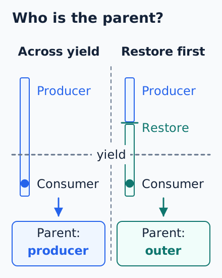
For that ownership model, activate the producer only around producer-owned
work. This async-generator excerpt accepts an iterable, a configured tracer
and a synchronous transform function:
from opentelemetry import trace


async def stream(items, tracer, transform):
    producer = tracer.start_span("produce")
    try:
        for item in items:
            with trace.use_span(producer, end_on_exit=False):
                value = transform(item)
            yield value  # no producer activation is suspended here
    finally:
        producer.end()
When iteration begins, start_span creates the producer under the then-current
outer context without activating it. Each use_span block activates that
existing producer only while transform() runs, so nested instrumentation
there can inherit it. end_on_exit=False matters: leaving the per-item
activation should not end the span describing the whole producer operation.
The with block exits before yield, restoring the outer parent. In Python's
contextvars-backed implementation, it also resets the attachment token in the
context that created it, rather than leaving a suspended activation for a
later cleanup task.
Resetting a token from another context can produce Failed to detach context.
That is application scope-lifetime misuse, not an unavoidable generator problem
or an SDK defect. Correct token cleanup alone does not guarantee the intended
parentage.
The finally block has a different responsibility: ending the producer on
completion, explicit closure or an error. The consumer must exhaust or close
the generator to establish that completion point. Losing interest in a stream
is not an adequate lifecycle protocol. This pattern separates the span's
duration from the smaller scopes in which it should influence parentage.
Context lifetime is also a memory question
Execution scope and object lifetime are separate concerns. A callback, task, or timer can retain context after the work that created it has finished. Ending a span does not necessarily release it from memory. Application references, active contexts, and other objects may keep it reachable.
For example, a retry registry that keeps obsolete timer handles can keep more than a small scheduling token alive. It can retain the context reachable from those handles. A garbage collector follows references; it does not treat "the request finished" or "the timer was cancelled" as instructions to discard objects that remain reachable.
In Node 24.15.0, deliberately retained timer handles still referenced their context frame and OpenTelemetry context after cancellation or completion. That shows why removing obsolete handles from an application registry matters. It establishes reachability, not a heap-byte estimate or a permanent leak.
Correlation identifiers and a whole context object also have different ownership costs. A log can carry a trace ID and span ID without keeping every value in the originating context alive. The logging handoff below shows an implementation that makes that separation explicitly.
Sources: Node 24.15.0 timer context capture, cancellation cleanup and completion cleanup.
Context propagation is not only about passing identifiers between operations. It also requires defining when a context becomes current, when that scope ends, and which objects may retain references after the operation finishes.
4. Why batching doesn't make everything asynchronous
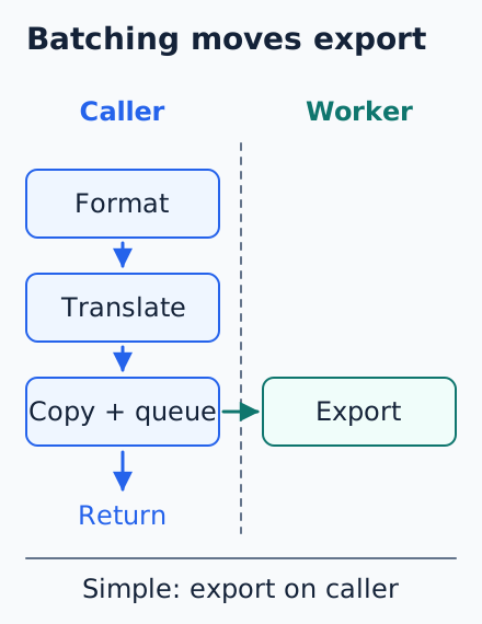
The import handler emits a log describing the completed job. You switch its pipeline to batch export, expecting telemetry work to leave the request thread. That expectation is partly right: export can move. It is the location of the handoff, rather than the word "batch," that determines what remains.
Before the queue, the caller still does the work
One common logging pipeline looks like this:
Application inputs -> logging API/bridge -> SDK processing -> queue admission -> worker -> exporter.
The application must evaluate its inputs before passing them to a logging call. The API or bridge turns those inputs into a record and invokes SDK processing. Within that path, the batch processor prepares and admits its queued representation. A worker later removes records and calls the exporter. That handoff is the point at which the caller can stop waiting for the export path; it does not make other configured processors asynchronous.
The exact location of formatting and conversion depends on the logging integration. A language's logging API may support lazy formatting or structured values, while its bridge decides how those become OpenTelemetry body, severity and attribute fields. Batching at the end of that preparation does not move the earlier stages along with export.
Consider the Python logging call logger.info("event=%s", build_event()).
The application builds the event before the logger receives it. With the
inspected logging bridge 0.66b1 and SDK 1.45.1, the enabled message-and-arguments
path creates a standard record, obtains its formatted message, translates it
and invokes the default processor chain on the emitting thread.
The logs specification requires processors to be invoked synchronously when a record is emitted. A processor may then hand work to a background worker, but its caller-side preparation still runs before that handoff.
In the inspected Python implementation, the batch processor prepares a copy of the log record before placing it in the queue. This work still happens on the emitting thread, even though export happens later.
The copy is shallow. The processor clears the copy's ambient context but keeps its correlation IDs, then wraps it as a readable record for the queue. The original remains available to other processors.
The same eager-evaluation trap from span attributes applies to logs.
Lazy %s formatting can defer stringification, but build_event() still
runs first. A level guard before construction avoids that unnecessary work
when the message is disabled.
Use a level check before expensive payload construction, not just lazy formatting around a value already built.
Trace sampling is a separate control. In the default Python logging pipeline examined here, an unsampled trace context does not automatically suppress its associated log record. If logs should follow trace-based filtering, that needs an explicit policy; a sampled-out trace is not automatically a log-off switch.
A full queue has to make a choice
The benefit of the handoff becomes clear when an exporter stalls. A simple processor can leave the sending thread waiting inside the exporter. A batch queue can let the producer continue while the worker waits. The queue separates caller progress from exporter progress, but only while its admission policy allows it.
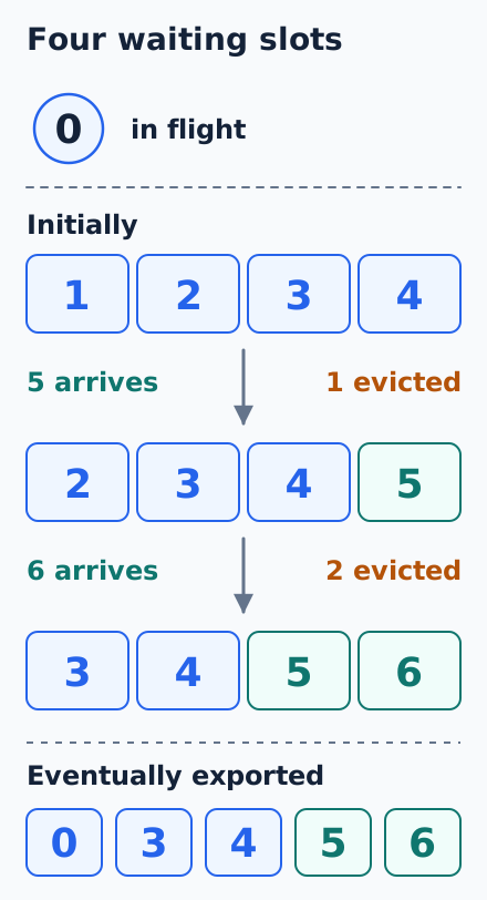
Once the queue fills, three policy families produce different failures. Rejecting a new arrival preserves the older backlog but loses the latest record. Evicting an old waiting record makes room for fresher data but discards earlier history. Blocking keeps pressure on the producer, which can now affect application latency or progress.
The Python SDK 1.45.1 example uses oldest-waiting eviction. One record is already in flight while four others fill the waiting slots. Two more arrivals replace the oldest waiting records. After the exporter resumes, the exported records are 0, 3, 4, 5, and 6.
A similar queue-admission trade-off appears in tracing: Go SDK 1.47.0's batch span processor rejects new spans when its queue is full by default, with an option to block producers instead. This is a comparison of admission policies across signals, not equivalent log processor implementations.
Four waiting slots therefore did not mean at most four records existed in the pipeline. Nor would a record-count limit describe their byte size: records with large bodies or attributes retain different amounts of data. Queue capacity, record size and in-flight work belong in the same memory discussion.
If records keep arriving faster than export can drain them, a larger queue buys time; it does not fix the sustained imbalance. It can also retain more record state and increase delivery delay. Blocking preserves backpressure at the cost of application progress. Dropping preserves application progress after some telemetry construction work has already been paid for.
Choose the policy deliberately and exercise it with a stalled exporter. Observe available drop and export-failure counters rather than deduplicated warnings. Healthy throughput does not describe behavior during the failure that makes the records most valuable.
Source: Go SDK 1.47.0 blocking and dropping admission paths.
Batching removes a dependency from the request path by accepting responsibility for work elsewhere. That work still needs a CPU, memory and a completion policy. The distinction becomes unavoidable when the service stops accepting requests but its queues and callbacks have not finished.
5. What happens when your application shuts down?
The import service receives a termination signal during a rolling restart. One handler has just ended its span, another is still streaming a response, and the batch worker is exporting a log. Teardown has three distinct steps.
First, stop admitting new application work. This prevents a moving target: there is little value in draining a pipeline while fresh requests continually create more work for it.
Next, finish the operations that can still produce telemetry within the application's completion budget. In the streaming example, the owner must finish or close the generator so its producer span ends. Final handlers may still emit logs or update metrics; shutting down their processors first would remove the path they expect to use.
Finally, shut down the telemetry pipeline through its documented lifecycle APIs while its dependencies remain available. Workers, executors, the runtime and transports may still be needed after the last response was sent. Closing those dependencies first can strand the work the shutdown operation must finish.
An empty queue is not a storage receipt
Queue admission says a record was accepted for later processing; it can still be evicted. Queue draining says nothing remains waiting there, but work may be in flight. Export completion means the export operation finished and reported a result that must be checked.
A worker removes a batch before its export operation returns. At that point the waiting queue can be empty while export is still running. Conversely, an exporter can consume a batch and return failure: completed execution and successful delivery are different observations. Queue length describes one container, not the state of the entire operation.
For a network exporter, success may mean that the destination acknowledged the data. It does not necessarily mean the data has been durably stored. That guarantee depends on what the destination promises.
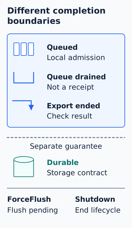
Flush requests completion; shutdown ends the lifecycle
ForceFlush asks for pending telemetry work to be completed. It does not
finish application operations that are still producing telemetry, and it
does not guarantee that a backend has durably stored the data.
Under the trace and log processor contracts, built-in processors must attempt pending exports and invoke exporter flush, subject to the timeout budget. These requirements apply to those processors, not every SDK component.
Calling flush while the streaming handler is still active does not make its eventual span ending part of the already-pending set. Nor does flush prevent another request from enqueueing a record afterward. It is not an application-wide barrier that stops new producers.
An explicit flush can be useful before an environment suspends a process. It is not intended to follow every recording call: repeatedly forcing small exports can undermine the batching you configured.
For those processors, Shutdown is terminal and must include the
effects of flush, so a separate flush-then-shutdown sequence is not universally
necessary. That inclusion rule should not be generalized to every reader or
exporter interface. Follow the documented lifecycle of the provider and
components being used; a shut-down processor is no longer available for
normal recording work.
Both operations can have blocking or asynchronous APIs. Wait for the documented completion result, not merely the call that initiates an asynchronous operation. Handle failures and timeouts explicitly.
Teardown has a finite resource budget
The service's grace period must cover application completion and telemetry teardown together. Independent timeouts that look reasonable in isolation can exceed that overall deadline when operations wait on one another.
The trace and log processor specifications prioritize an explicit flush timeout over finishing every export call. A finite shutdown budget can therefore trade complete delivery for bounded termination. Work out which layer enforces the deadline: stopping the caller's wait, stopping worker work and cancelling a transport operation are not automatically the same event.
The three-step ordering keeps ownership clear; it cannot promise lossless delivery within an arbitrary grace period. Decide how the application and telemetry pipeline share that deadline, how completion failures are surfaced, and what happens to work left over when the process must exit.
Where did the cost move?
A larger application memory footprint does not, by itself, mean the whole telemetry pipeline became more expensive. SDK work counts against the application's budget; agents, transport and backends have their own costs.
Moving aggregation out of the application requires a transport that carries individual measurements to another process. Putting a Collector after aggregated OTLP export does not remove the SDK work that produced it.
Aggregating here or sending measurements elsewhere
Consider a service recording request durations. Application measurements update in-process SDK histogram buckets and related state. With an OTLP exporter, the SDK sends aggregated metrics to a Collector or backend. The application pays for that state and the work of updating it.
An alternative architecture sends individual measurements through a measurement-capable transport to an agent. The agent aggregates them and exports aggregated metrics to a backend.
The handoff is before aggregation rather than after it. The application still constructs attributes and prepares transport input, and that input path must decide whether to buffer, drop or block when the agent is unavailable or slow.
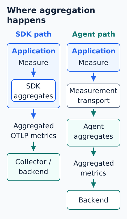
Combining many measurements for one series can reduce network traffic and downstream work, even though it requires application memory. The metric data model supports preaggregated streams and downstream reaggregation.
For the import service's bounded outcome counter, many requests update a few entries before collection. Sending each measurement to an agent instead puts more individual work across the transport boundary. A fresh request ID on every measurement offers little opportunity to combine updates; moving that state does not bound its cardinality.
Compare cardinality, collection intervals and payload sizes along with the agent's own CPU, memory and transport work. Moving aggregation must also preserve metric identities, histogram semantics and reset behavior.
Exporting now or handing work to a queue
Batching can move export off the caller's path, exchanging caller waiting for queue memory and later delivery. Caller-side formatting and admission stay where they were; worker CPU still counts toward application overhead.
Larger batches can amortize export overhead, but add delay. Serialization, transport, retries and the queue's loss or backpressure policy still belong in the whole-system comparison.
Follow execution, state and completion
Where does the work execute? A worker moves scheduling within the application; an agent moves work across a process boundary. Application overhead concerns the service's CPU, memory and request latency. Total pipeline cost also includes agents, transport processing and backend work. A smaller application profile can mean another component now pays more.
Who owns retained state? Identify the owners of aggregation entries, instrument registries, queues and context references, and the condition that releases each one. Moving an unbounded identity space to an agent changes where it consumes memory, not whether it needs a bound.
Who is responsible for completion or loss? Ask where unfinished telemetry lives if the application exits, what an agent restart can lose, and which component applies backpressure. Process separation can isolate some failures, but not shared-host exhaustion. Buffering and acknowledgement contracts still determine what progress means across that boundary.
Neither architecture is automatically cheaper. Comparing them fairly requires measuring costs across the entire telemetry pipeline.
Instrumentation belongs in the application's design
Instrumentation is part of an application's execution path, memory model, and lifecycle. Sampling, aggregation, and batching change how telemetry is processed, but they do not make its earlier costs disappear. To understand the real cost of observability, look beyond what reaches the backend and examine what the application must do, retain, and eventually complete.
Keep following the thread.
Back to all articles